Mean, Median & Mode – Which “Average” Should We Trust?

Before we start, let me answer the small challenge from the last diary entry:

Is a postal code qualitative or quantitative?

It is qualitative. A postal code is written with numbers, but it is really a label for an area. It does not measure “how much” of anything. You can calculate an “average postal code”, but the result means nothing. It is like calculating the average of phone numbers.

I like this example because it teaches something bigger: the numbers are not the whole story. We also need to understand what the numbers mean.

And that is exactly the topic of today’s entry.

The word we use every day

We use the word “average” all the time:

• the average salary
• the average house price
• the average exam score
• the average waiting time

It sounds simple. But when I started learning statistics, I was surprised to find out that there is more than one kind of average.

In statistics, the three most common ones are the mean, the median, and the mode. All three try to describe the center of the data: what is “typical”. But they do it in different ways.

Sometimes they give almost the same answer. Sometimes they give very different answers. And when they are very different, the data is usually trying to tell us something.

Let’s meet them one by one.

Mean: the one we already know

The mean is what most people call “the average”.

To find it, we add all the values and divide by how many values there are.

Imagine five students get these scores:

70, 75, 80, 85, 90

• Add them: 70 + 75 + 80 + 85 + 90 = 400
• Divide by 5: 400 ÷ 5 = 80

Mean = sum of all values ÷ number of values

The mean is useful because it uses every value in the data. But this strength is also its weakness. If one value is very big or very small, it can pull the mean away from what is typical. We will see this very soon.

Median: the one in the middle

The median is the middle value after we put the data in order, from smallest to largest.

Example:

5, 7, 9, 12, 20

The value in the middle is 9. So the median is 9.

What if there is an even number of values? For example:

5, 7, 9, 12

Now there are two middle values: 7 and 9. We take the mean of these two:

(7 + 9) ÷ 2 = 8

So the median is 8.

The important thing: the median depends on the position of the values, not on how big the extreme values are. If I change 20 to 2,000 in the first example, the median is still 9. This makes the median very useful when the data has some unusual values.

Mode: the most popular one

The mode is the value that appears most often.

Here are the shoe sizes of a small group:

39, 40, 40, 41, 41, 41, 42

Size 41 appears three times, more than any other size. So the mode is 41.

A dataset can have one mode, more than one mode, or no mode at all (if every value appears only once).

The mode has one special power: it also works with categories (the qualitative data from our last entry). Imagine 100 customers choose their favorite payment method: cash, credit card, bank transfer, or mobile payment. We cannot calculate a “mean payment method”. It makes no sense. But we can find the mode: the method that most people chose.

🔍 For the curious: For continuous data (like height measured very precisely), almost every value is different, so the simple mode is not very useful. In that case, we usually group the data into ranges and look for the most common range. A dataset with two clear peaks is called bimodal. This often means there are two different groups mixed together, for example the shoe sizes of both adults and children.

The drama: seven coworkers and one salary question

Now let’s see why these three measures can tell very different stories.

Imagine a small office with seven people. Their monthly salaries, in million VND, are:

Person	A	B	C	D	E	F	Owner
Salary (mil VND)	8	8	9	10	10	10	60

Six people earn between 8 and 10 million. The owner earns 60 million.

Let’s calculate.

Mean:
8 + 8 + 9 + 10 + 10 + 10 + 60 = 115
115 ÷ 7 ≈ 16.4 million VND

Median: The data is already in order. With seven values, the middle one is the 4th value: 10 million VND.

Mode: 10 appears three times, more than any other value: 10 million VND.

Measure	Result
Mean	≈ 16.4 million VND
Median	10 million VND
Mode	10 million VND

Same data. Different answers.

Now imagine a job advertisement says: “The average salary in our office is 16.4 million VND!”

Is it true? Yes, mathematically, it is 100% correct.

But is it honest? Not really. Nobody except the owner earns close to 16.4 million. A new employee who reads this advertisement will expect much more than they will actually get.

This was a big lesson for me: a number can be correct and still give the wrong picture.

One very high salary pulled the mean up. A value that is much higher or lower than the rest is called an outlier. The median and the mode did not move much because of the outlier, so they describe a “typical” employee much better here.

This is why official statistics about income and house prices often report the median, not the mean.

🔍 For the curious: In statistics, a measure that is not easily affected by outliers is called robust. The median is robust; the mean is not. There is also a middle option called the trimmed mean: we remove a small percentage of the highest and lowest values, then calculate the mean of the rest. Some sports use this idea, for example when judges’ highest and lowest scores are removed.

“The average salary went up 35%!” — Which average?

Let’s continue the story. Next year, nobody in the office gets a raise, except the owner. His salary goes from 60 to 100 million VND.

New data: 8, 8, 9, 10, 10, 10, 100

• New mean: 155 ÷ 7 ≈ 22.1 million VND (up about 35%!)
• New median: still 10 million VND (no change)

So the owner could say: “The average salary in our company increased by 35% this year!”

Again, this is mathematically true. But six out of seven people got nothing.

So now, every time I read “the average went up”, I try to ask:

• Which average: mean or median?
• Did most people get better, or only a few?
• What does the data look like behind this one number?

So, which one should we use?

There is no single right answer. It depends on the data and on what we want to understand.

Use the…	When…	Examples
Mean	The values are fairly balanced, with no extreme outliers	Exam scores, daily temperature, daily sales
Median	Some values are much higher or lower than the rest	Salaries, income, house prices, waiting times
Mode	We want to know what is most common, or the data is categories	Shoe sizes, most popular product, favorite payment method

A small clue hidden in the numbers

Here is a habit I am trying to build:

When the mean and the median are very different, ask why.

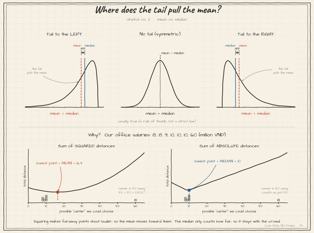
A big difference often means there are outliers, or that the data stretches much further in one direction than the other. This is called a skewed distribution. Our salary data is a good example: most values are small, and one value is far out to the right.

We will look at the shape of data more carefully later in this series. For now, just remember: the gap between the mean and the median is itself a small piece of information.

🔍 For the curious: When data has a long tail to the right (like income), the mean is usually larger than the median. When the tail goes to the left, the mean is usually smaller. This is a useful rule of thumb, but not a strict law; there are exceptions. There is also a deeper difference: the mean is the value that makes the sum of squared distances to all data points as small as possible, while the median makes the sum of absolute distances as small as possible. This is one reason the mean reacts much more strongly to faraway values.

Today I learned

1. Mean = add all values and divide by how many values there are.
2. Median = the middle value after putting the data in order.
3. Mode = the value that appears most often. It also works for categories.
4. Outliers can pull the mean up or down, but the median is much less affected.
5. The “best” average depends on the data. When the mean and median are very different, ask why.

Quick check

Five houses on the same street were sold for (in million Baht):

2.0, 2.1, 2.2, 2.3, 9.0

Which number better describes the price of a typical house on this street: the mean or the median?

Mean = (2.0 + 2.1 + 2.2 + 2.3 + 9.0) ÷ 5 = 17.6 ÷ 5 = 3.52 million baht
Median = 2.2 million baht
Four of the five houses cost between 2.0 and 2.3 million baht. The 9-million-baht house pulls the mean up. So the median gives a better picture of a typical house here.

Click to see the answer

A small challenge before next time

Outliers are not always big. Look at these exam scores:

20, 85, 88, 90, 92

Calculate the mean and the median. Which direction did the outlier pull the mean? And if you were the teacher, which number would you report to describe the class?

Write your answer in the comments!

One final thought

Mean, median, and mode are some of the simplest ideas in statistics. But simple does not mean unimportant. The way we summarize data can completely change the story people see.

So the next time you see the word “average”, maybe ask one small question:

“Which average?”

Behind one simple number, there is often a much more interesting story.

In the next diary entry, we will look at something the average cannot show us at all: how spread out the data is. Two classes can have the same average score, and still be very, very different.

See you in the next diary entry!